|
Search DSS Finding Data Analyzing Data Citing data About Us DSS lab consultation schedule (Monday-Friday)
*No appts. necessary during walk-in hrs. Note: the DSS lab is open as long as Firestone is open, no appointments necessary to use the lab computers for your own analysis.  
|
Home Interpreting Regression Output
IntroductionThis guide assumes that you have at least a little familiarity with the concepts of linear multiple regression, and are capable of performing a regression in some software package such as Stata, SPSS or Excel. You may wish to read our companion page Introduction to Regression first. For assistance in performing regression in particular software packages, there are some resources at UCLA Statistical Computing Portal. Brief review of regressionRemember that regression analysis is used to produce an equation that will predict a dependent variable using one or more independent variables. This equation has the form
where Y is the dependent variable you are trying to predict, X1, X2 and so on are the independent variables you are using to predict it, b1, b2 and so on are the coefficients or multipliers that describe the size of the effect the independent variables are having on your dependent variable Y, and A is the value Y is predicted to have when all the independent variables are equal to zero.
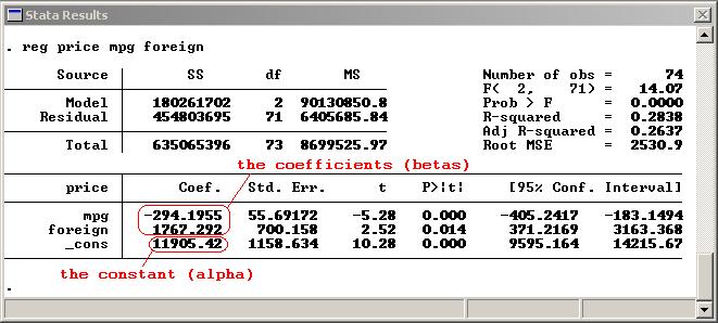
In the Stata regression shown below, the prediction equation is price =
-294.1955 (mpg) + 1767.292 (foreign) + 11905.42 - telling you that price
is predicted to increase 1767.292 when the foreign variable goes up by
one, decrease by 294.1955 when mpg goes up by one, and is predicted to be
11905.42 when both mpg and foreign are zero.
Coming up with a prediction equation like this is only a useful exercise if the independent variables in your dataset have some correlation with your dependent variable. So in addition to the prediction components of your equation--the coefficients on your independent variables (betas) and the constant (alpha)--you need some measure to tell you how strongly each independent variable is associated with your dependent variable. When running your regression, you are trying to discover whether the coefficients on your independent variables are really different from 0 (so the independent variables are having a genuine effect on your dependent variable) or if alternatively any apparent differences from 0 are just due to random chance. The null (default) hypothesis is always that each independent variable is having absolutely no effect (has a coefficient of 0) and you are looking for a reason to reject this theory. P, t and standard errorThe t statistic is the coefficient divided by its standard error. The standard error is an estimate of the standard deviation of the coefficient, the amount it varies across cases. It can be thought of as a measure of the precision with which the regression coefficient is measured. If a coefficient is large compared to its standard error, then it is probably different from 0. How large is large? Your regression software compares the t statistic on your variable with values in the Student's t distribution to determine the P value, which is the number that you really need to be looking at. The Student's t distribution describes how the mean of a sample with a certain number of observations (your n) is expected to behave.
If 95% of the t distribution is closer to the mean than the t-value on the coefficient you are looking at, then you have a P value of 5%. This is also reffered to a significance level of 5%. The P value is the probability of seeing a result as extreme as the one you are getting (a t value as large as yours) in a collection of random data in which the variable had no effect. A P of 5% or less is the generally accepted point at which to reject the null hypothesis. With a P value of 5% (or .05) there is only a 5% chance that results you are seeing would have come up in a random distribution, so you can say with a 95% probability of being correct that the variable is having some effect, assuming your model is specified correctly. The 95% confidence interval for your coefficients shown by many regression packages gives you the same information. You can be 95% confident that the real, underlying value of the coefficient that you are estimating falls somewhere in that 95% confidence interval, so if the interval does not contain 0, your P value will be .05 or less. Note that the size of the P value for a coefficient says nothing about the size of the effect that variable is having on your dependent variable - it is possible to have a highly significant result (very small P-value) for a miniscule effect. CoefficientsIn simple or multiple linear regression, the size of the coefficient for each independent variable gives you the size of the effect that variable is having on your dependent variable, and the sign on the coefficient (positive or negative) gives you the direction of the effect. In regression with a single independent variable, the coefficient tells you how much the dependent variable is expected to increase (if the coefficient is positive) or decrease (if the coefficient is negative) when that independent variable increases by one. In regression with multiple independent variables, the coefficient tells you how much the dependent variable is expected to increase when that independent variable increases by one, holding all the other independent variables constant. Remember to keep in mind the units which your variables are measured in. Note: in forms of regression other than linear regression, such as logistic or probit, the coefficients do not have this straightforward interpretation. Explaining how to deal with these is beyond the scope of an introductory guide. R-Squared and overall significance of the regressionThe R-squared of the regression is the fraction of the variation in your dependent variable that is accounted for (or predicted by) your independent variables. (In regression with a single independent variable, it is the same as the square of the correlation between your dependent and independent variable.) The R-squared is generally of secondary importance, unless your main concern is using the regression equation to make accurate predictions. The P value tells you how confident you can be that each individual variable has some correlation with the dependent variable, which is the important thing. Another number to be aware of is the P value for the regression as a whole. Because your independent variables may be correlated, a condition known as multicollinearity, the coefficients on individual variables may be insignificant when the regression as a whole is significant. Intuitively, this is because highly correlated independent variables are explaining the same part of the variation in the dependent variable, so their explanatory power and the significance of their coefficients is "divided up" between them. Further Reading |